
Having worked at the support desk here at Bench-Mark since 2017, I have gotten a lot of different questions over the years on all manner of things related to surveying with RTK equipment. A lot of these questions inspire our articles and especially the videos we film. And although I get a lot of different ones, on everything from is tilt really faster (Hemisphere S631: Does Tilt Make You Faster?) to how do I increase the range on my internal radios (Hemisphere S631: Radio Range) one of the most common questions I get is a question surrounding how long a point should be averaged for. In fairness it is a great question, if you can shave even 2 observations off of a point occupation, over 300 points that is 2.5 minutes. Over the course of the year that can be hours and hours in the field saved.
However, in the field of surveying and geospatial data collection, efficiency and precision go hand in hand. We can’t sacrifice precision at the feet of efficiency. Similar to our: Are You Recording Static Properly test, we are going to set out to determine what the optimal averaging time interval is to achieve optimal precision. For more on the difference between accuracy and precision, check out our article: Surveying With RTK: What is the Difference Between Accuracy and Precision?
Time is money in the field, and unnecessary delays can significantly impact productivity. So, in this article, I am going to explain why we can increase our precision by averaging observations, how we can test if this is the case, and if there is actually an averaging interval where the increased observation time is no longer worth the increased precision. With this information you can better optimize your equipment to perform your surveys better. If you would rather watch my video on this topic, check out the link below (although I get a little more in depth in this article).
Understanding GPS Error and Averaging
How Averaging Points Improves Precision
Does Averaging Points Actually Make A Difference: The Results
Practical Implications for Surveyors
As the name suggests, Averaging points involves collecting multiple observations over a period of time and combining them to determine a more precise position. This method is widely recommended by state boards and federal agencies to minimize positional errors. In fact, as per Natural Resource Canada (NRCAN) guidelines:
Control points should use a time window average of at least 1-minute, topographic points at least 5 seconds, and until the desired QC indicators are achieved. For topographic surveys, the use of this 5 second window average will reduce the effect of individual coordinate solution variations. For precise work such as control station establishment, longer time windows of up to 5 minutes should be used.1 (You can see the references at the end of this article for this report and the studies NRCAN referenced).
There are often legal reporting guidelines that have to be followed and these guidelines underscore the importance of averaging, particularly for high-precision applications. However, understanding how GPS error works can help us determine whether additional time spent averaging is truly beneficial beyond a certain threshold.
How Error Works
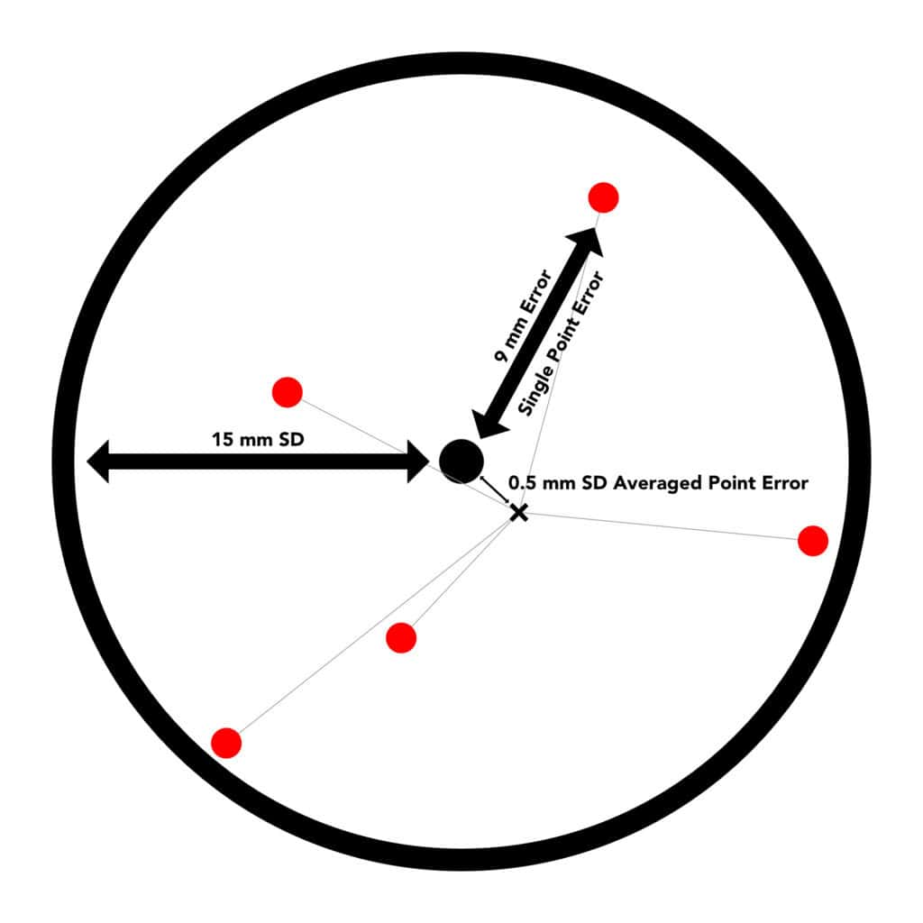
Before we get into the results of our test, we need to first understand how measurement error works. GPS observations are subject to various sources of error, including atmospheric interference, satellite geometry, and receiver noise. When a single point observation is taken, it does not necessarily land precisely at the true location. This is why when you read specification sheet, accuracy is reported as +/- 15 mm + 1 ppm. With this notation your coordinate is statistically supposed to be within 15 mm in any direction from your true coordinate, with an additional 1 mm added for every kilometer you are from the base.

This metric in GPS accuracy is known as confidence interval. It is expected that 95% of your recorded coordinates will be within 15 mm of the true position. This error can be mapped as a distribution of error. For GNSS this error distribution can be effectively shown using a Gaussian Distribution. Keep in mind this assumes no user or systematic errors, ie misplaced pole points, or out of level poles, or multi-path effects (which for our purposes we are going to assume that we are perfect surveyors).
What is a Gaussian or Normal Distribution?
For many types of error in the world we can observe a gaussian or normal distribution. This kind of error is purely random, so that if the experiment is repeated over and over again, the distribution of the results when plotted will resemble a bell curve, which is known as a Gaussian distribution.2

A Gaussian distribution plots the number of instances of a specific measurement occurring. If an error is random and normally distributed, observations will be most common near the mean, becoming less and less likely as we move further away. Classic examples in everyday life include height and birth weight of babies.
The smaller the standard deviation, the more precise the results. Ideally, by averaging the points we are going to produce tighter standard deviation and therefore be able to achieve a higher degree of precision. You can read more about the math behind these distributions here: The Normal Distrbution (USU).
We are able to theoretically improve precision by averaging multiple observations together. Through averaging multiple points, extreme outliers in the dataset are smoothed out.
In order to see how the length of measurement effects the precision of the position, we used the testing parameters found here: How Repeatable is RTK GPS in the Real-World.
Now for our test, we obviously need to record for intervals longer than 1 second. To keep things consistent, we used a 5:05 interval between shots. This allowed us to record the 5-minute observation window without having the number of observations be different between our time intervals. Otherwise, testing parameters were the same as our repeatability test. We used the same position, same receiver and same data collector. For our test we used the following time intervals and observation number:
| Number of Averaged Points in Observation | Number of Recorded Points |
| 5 | 101 |
| 15 | 67 |
| 30 | 101 |
| 60 | 91 |
| 180 | 78 |
| 300 | 103 |
For 15 and 180 seconds, connection to the data collector was lost and the receiver had to be reconnected resulting in lost time during collection. We can than compare the collected averaged positions and compare them to one another to see if the averaging does in fact increase precision. If it does, we should see an increase in the precision and a decrease in the standard deviation.
Our test position as shown in the video is in a relatively open environment. There is a set of trees (with no leaves) and powerline approximately 40 ft to the North East, and a building approximately 20 ft to the South West. Otherwise, conditions are open above the receiver. There should be limited multi-path conditions.
For my testing today, I used a Hemisphere S631, a Juniper Mesa 3 data collector and MicroSurvey’s FieldGenius Windows. As the Auto-Record function only allows for 1s observations, I used an auto-clicker to press the store point button.
Vertical Data
I am going to first look at the vertical data, as vertical data has the largest standard deviation. This has to do with a number of mathematical functions and the position of the satellites. You can read more here on why that is: GNSS Error Sources.3
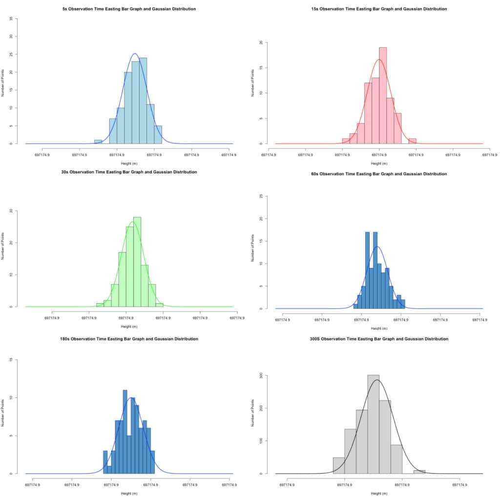
The first thing we should check is whether or not our error was normally distributed.
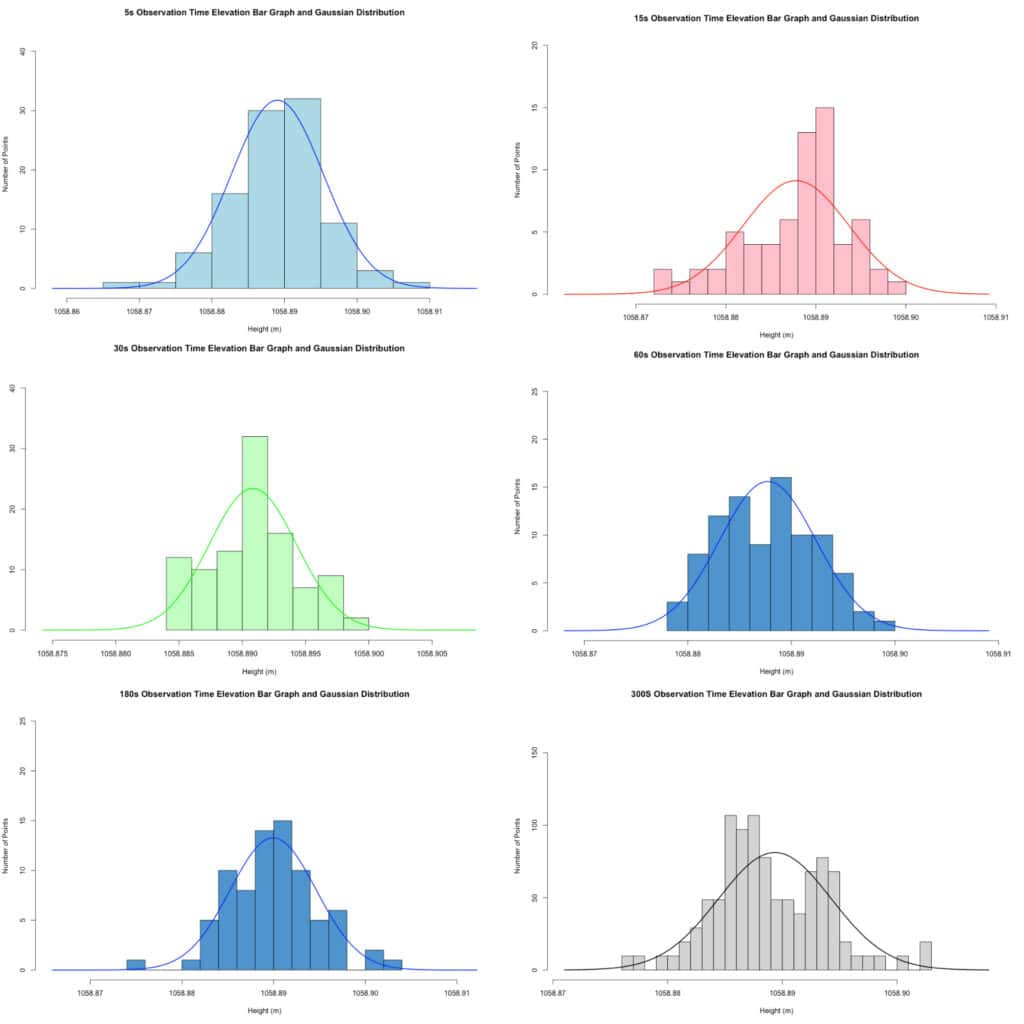
As we can see from the results, all of our time intervals follow the expected Gaussian error distribution. With more observations, it can be expected that the bar graphs would more closely begin to resemble the Gaussian curve.
| Number of Observations | Total Number of Points | Standard Deviation (+/- mm) |
| 5 | 101 | 6.37 |
| 15 | 67 | 5.90 |
| 30 | 101 | 3.46 |
| 60 | 91 | 4.68 |
| 180 | 78 | 4.71 |
| 300 | 103 | 4.94 |
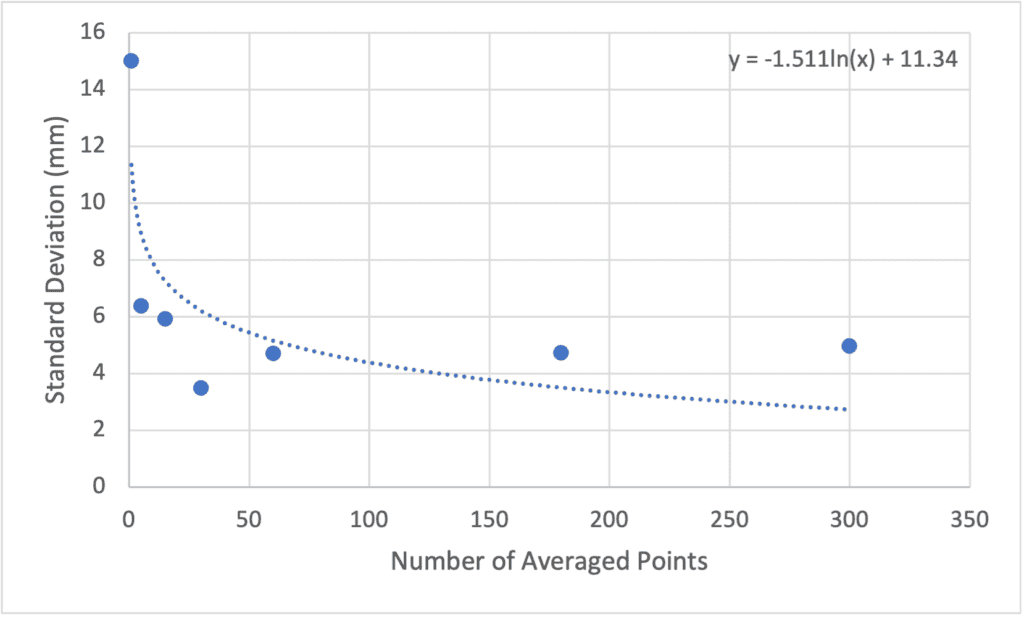
As expected, over our sample size, we saw an increase in precision as the number of observations was increased. From our sample and in our conditions, it appears that after 30 seconds, there is not a huge increase in precision, relative to the increase in time it takes to record the position. However, over a 1,000 or 10,000 shot sample this may become more dramatic.
Northing Data
In our X and Y coordinates, we should see a less dramatic effect. This is because on a single point observation, we are expecting a +/- 8 mm difference in position.
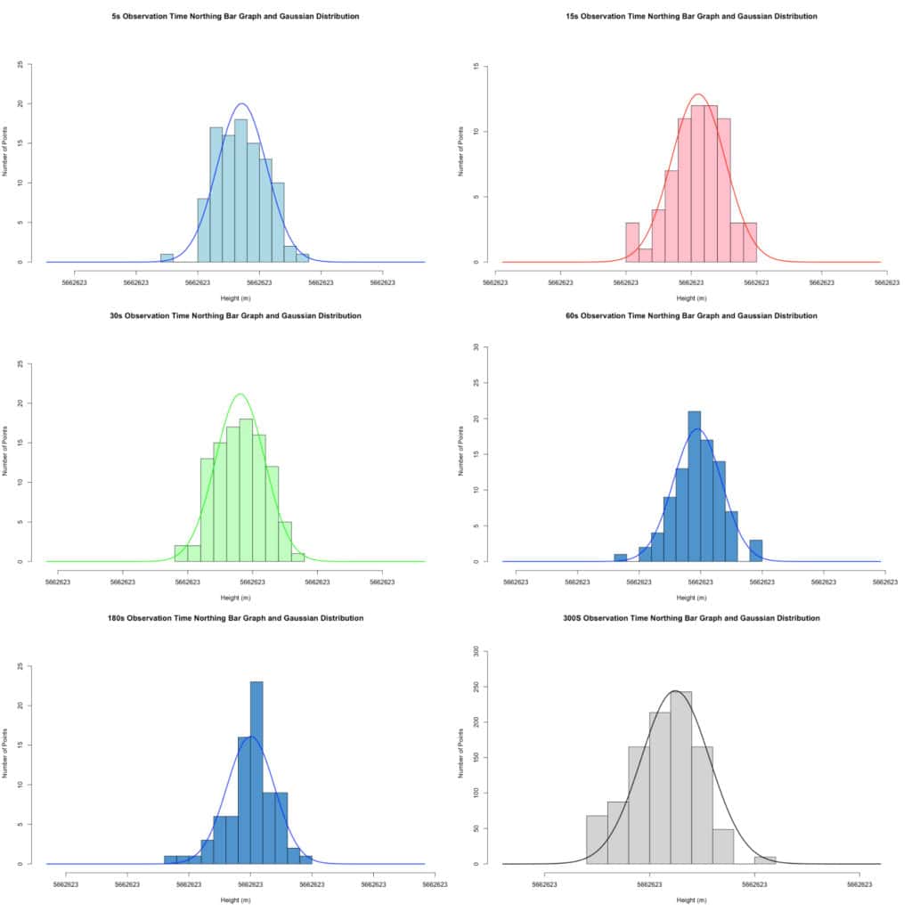
| Number of Observations | Total Number of Points | Standard Deviation (+/- mm) |
| 5 | 101 | 2.02 |
| 15 | 67 | 2.09 |
| 30 | 101 | 1.91 |
| 60 | 91 | 1.96 |
| 180 | 78 | 1.94 |
| 300 | 103 | 1.64 |
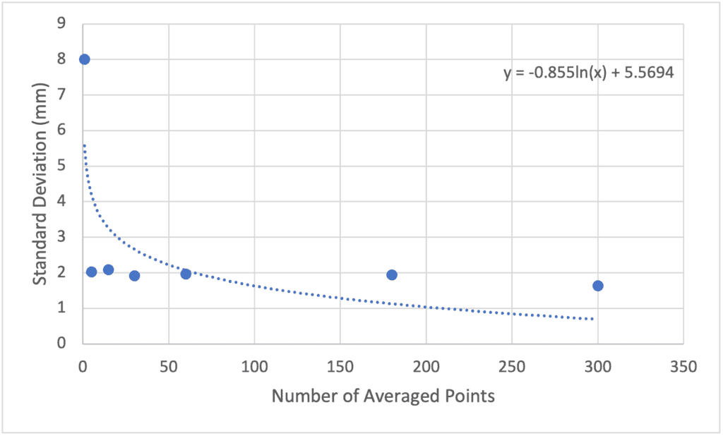
Unlike with the vertical, it appears that the precision increase you achieve is less significant. Over the approximately 100s sample, there is no statistical difference between the 5 and 300 s observation.
Easting Data
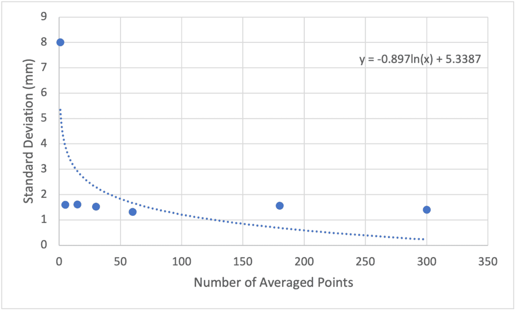
A similar story is found in the Easting data. We again have normally distributed data, but there is no large increase in precision from taking more observations.
| Number of Observations | Total Number of Points | Standard Deviation (+/- mm) |
| 5 | 101 | 1.60 |
| 15 | 67 | 1.61 |
| 30 | 101 | 1.52 |
| 60 | 91 | 1.32 |
| 180 | 78 | 1.56 |
| 300 | 103 | 1.40 |
For surveyors and engineers in the field, the key takeaway is that increasing averaging time improves accuracy, but only up to a certain point. These results should only be used to help inform you of your options, many states and provinces have regulatory and reporting requirements. Many state boards and federal agencies mandate minimum observation times for specific applications and points. I would always recommend checking in with your local state board for their recommendations. The results we tested here are only valid for our conditions, and may vary based on where you are and if you are in multi-path conditions. If you are in more difficult conditions with a large amount of obstacles that could cause multi-path conditions, you may want to increase the number of observations in your averaging window.
Several of the mathematical concepts in this article (Gaussian distributions, standard deviation, confidence intervals) are part of the broader set of land surveying equations that inform how we interpret our data. Understanding the equations behind the numbers helps you make better decisions in the field.
Standard Deviation measures the spread of observations around the mean. The smaller the standard deviation, the more precise your survey. In our test, this is exactly what we measured, reducing vertical standard deviation from 6.37 mm at 5 observations down to 3.46 mm at 30.
Standard Error of the Mean (SE = σ / √n) explains why averaging more observations improves precision. As n increases, the standard error shrinks. It also explains the diminishing returns: doubling your observations doesn’t halve your error because the relationship is governed by a square root function.
Confidence Intervals are what the +/- 15 mm figure on a GNSS specification sheet represents, the range within which 95% of observations are expected to fall. This is why averaging tightens the interval around your true position.
In day-to-day RTK work, your field software handles all of this automatically. But knowing what the numbers mean helps you set appropriate averaging windows, interpret your QC indicators correctly, and recognize when something in the field is a genuine issue versus normal statistical variation.
GPS point averaging is an essential technique for improving precision in fieldwork. However, excessive averaging can lead to unnecessary delays. The key findings from this test suggest that a 30-second observation window strikes the optimal balance between accuracy and efficiency in the vertical, while a 5 s observation window can be sufficient in the horizontal. Beyond this threshold, additional time spent averaging may not lead to an equal increase in precision..
For surveyors, engineers, and geospatial professionals, understanding these dynamics allows for smarter decision-making in the field. By applying these insights, fieldwork can be completed more efficiently without compromising accuracy, ultimately saving both time and resources.
If you have any questions or comments, reach out to me at [email protected]!
(1) Danahue, B.; Wentzel, J.; Berg, R. Guidelines for RTK/RTN GNSS Surveying in Canada; 2015. https://natural-resources.canada.ca/sites/nrcan/files/earthsciences/pdf/Canada%20RTK_UserGuide_v1_2-EN.pdf (accessed 2025-02-17).
(2) Harris, D. C.; Lucy, C. A. Quantitative Chemical Analysis, 9th ed.; W.H. Freeman Company, 2016.
(3) Karaim, M.; Elsheikh, M.; Noureldin, A. GNSS Error Sources. In Multifunctional Operation and Application of GPS; InTech, 2018; pp 69–85. https://doi.org/10.5772/intechopen.75493
Bench Mark Equipment & Supplies is your team to trust with all your surveying equipment. We have been providing high-quality surveying equipment to land surveyors, engineers, construction, airborne and resource professionals since 2002. This helps establish ourselves as the go-to team in Calgary, Canada, and the USA. Plus, we provide a wide selection of equipment, including global navigation satellite systems, RTK GPS equipment, GNSS receivers, and more. We strive to provide the highest level of customer care and service for everyone. To speak to one of our team today, call us at +1 (888) 286-3204 or email us at [email protected]